What you’ll learn

• what a cluster is, and why the definition is a choice rather than a fact
• three distance metrics, computed by hand on the same pair of points
• why scaling changes the answer, measured: ARI 0.035 → 0.891
• the silhouette coefficient, derived and computed by hand
• three internal validation scores, and what each one rewards
• why “how many clusters?” has no purely mathematical answer

Intuition

Every supervised page so far had an answer key. You fit a model, compared its predictions with yy, and got a number. Clustering has no yy. You hand an algorithm a matrix of features and it hands back a group label for each row, and there is nothing to check it against.

That sounds like it should make clustering easier — no labels to collect, no leakage to worry about. It makes it harder, because the question “is this grouping right?” has no answer. It has only the question behind it: right for what?

Consider six people described by two numbers, age and annual income:

There are two obvious groupings. By age: $\{A, B, C\}$ and $\{D, E, F\}$. By income: everyone in one group, because incomes barely differ. Both are defensible. Which one an algorithm returns is decided entirely by how you measure “close” — and that decision is made before the algorithm runs, by the units your columns happen to be in.

That is the single most important fact on this page. Clustering algorithms do not find structure. They find the structure implied by your distance metric.

  flowchart LR
  X["Unlabelled X"] --> M["Choice of distance metric
(and scaling)"]
  M --> A["Clustering algorithm"]
  A --> L["Group labels"]
  L --> V["Internal validation
silhouette, Davies-Bouldin, ..."]
  V -->|"score is low"| M
  V -->|"score is fine but
the groups are useless"| Q["Wrong question.
Change the features."]

The math

A metric on a feature space is a function $d(\mathbf{x}, \mathbf{y})$ satisfying four properties: it is non-negative, it is zero exactly when the points coincide, it is symmetric, and it obeys the triangle inequality

Three metrics cover almost everything you will use.

Euclidean distance (the $L_2$ norm) is straight-line distance:

Manhattan distance (the $L_1$ norm) is the distance walked along the axes:

Cosine distance ignores magnitude entirely and measures only the angle between the two vectors:

Cosine distance is not a true metric — it violates the triangle inequality — but it is the right choice whenever the direction of a vector carries the meaning and its length does not. Document term-frequency vectors are the standard example: a 200-word article and a 2,000-word article about the same topic point the same way but have wildly different lengths.

Both $L_1$ and $L_2$ are special cases of the Minkowski distance:

with $q = 1$ and $q = 2$. As $q \to \infty$ this converges to the Chebyshev distance, $\max_j |x_j - y_j|$.

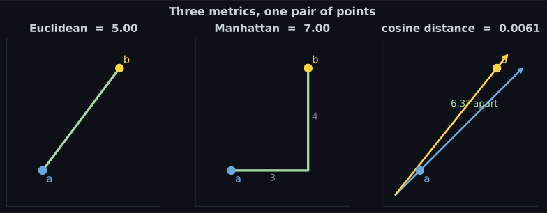
Worked example by hand

Take $\mathbf{a} = (1, 1)$ and $\mathbf{b} = (4, 5)$. The differences are $3$ and $4$.

Euclidean:

Manhattan:

Cosine: the dot product is $1 \cdot 4 + 1 \cdot 5 = 9$. The norms are $\lVert \mathbf{a} \rVert = \sqrt{2} = 1.41421$ and $\lVert \mathbf{b} \rVert = \sqrt{41} = 6.40312$.

which corresponds to an angle of $6.34°$. By Euclidean distance these points are five units apart — substantial. By cosine distance they are practically identical, because they point almost the same way from the origin. Same two points, two completely different verdicts.

figureThree metrics, one pair of pointsmatplotlib

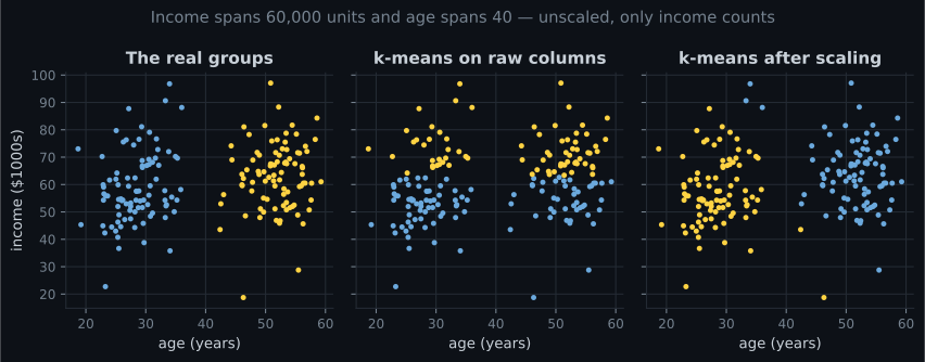
Scaling decides the answer

Here is the failure the six-person table hinted at, run for real on 180 people. Ages are drawn from two groups centred on 28 and 52; incomes are drawn from two nearly identical distributions centred on 60,000 and 64,000. The genuine structure is entirely in the age column.

The raw column standard deviations are 12.3 years and 12,698 dollars. Squared Euclidean distance adds those contributions together, so the income term is about a million times larger. The age column is arithmetically invisible.

figureThe same data, clustered twicematplotlib

Scale your features before clustering, unless you have a specific reason not to. The exception is when the units are already comparable and the relative spread is meaningful — pixel intensities, or a set of columns all measured in dollars.

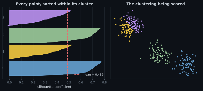
Scoring a clustering without labels

You cannot compute accuracy without an answer key, but you can ask whether the groups are internally tight and mutually far apart. Three scores do this.

The silhouette coefficient

For a single point $i$ in cluster $C_I$, define

• $a(i)$ = mean distance from $i$ to the other points in its own cluster (how tight it sits),
• $b(i)$ = the smallest mean distance from $i$ to all points of any other cluster (how far it is from the nearest rival).

Then

If $|C_I| = 1$ the convention is $s(i) = 0$. Reading the value:

• $s(i)$ near $+1$: much closer to its own cluster than to any other — well placed.
• $s(i)$ near $0$: sits on the boundary between two clusters.
• $s(i)$ negative: closer, on average, to a different cluster than to its own — misassigned.

The silhouette score of a clustering is the mean of $s(i)$ over every point.

Worked silhouette, by hand

Five points on a line: $x = 1, 2, 3$ in cluster 0, and $x = 10, 11$ in cluster 1. Take the point at $x = 2$.

Its own cluster contains $1$ and $3$, both at distance 1:

The other cluster contains 10 and 11, at distances 8 and 9:

Now take the point at $x = 3$, which sits at the edge. $a = (2 + 1)/2 = 1.5$ and $b = (7 + 8)/2 = 7.5$, so $s = 6/7.5 = 0.8$. Lower, as it should be — that point is nearer the other group.

The other two

Davies-Bouldin index. For each cluster, find the worst-case ratio of “sum of the two clusters’ average internal spread” to “distance between their centroids”, then average those worst cases:

Lower is better, and 0 is perfect. This is the one score on this page where a smaller number means a better clustering — a common source of sign errors.

Calinski-Harabasz index (the variance-ratio criterion) is between-cluster dispersion over within-cluster dispersion, scaled by the degrees of freedom:

Higher is better. It is by far the cheapest of the three — $O(n)$ rather than the silhouette’s $O(n^2)$ — which matters once $n$ passes a few tens of thousands.

All three assume clusters are roughly round blobs. On the two-moons dataset, a correct clustering scores worse than a wrong one on all three. Internal scores are a tool for comparing runs on similar geometry, not a verdict on truth.

figureReading a silhouette plotmatplotlib

See it move

And here is the metric choice made tangible — drag the slider by clicking, and watch which pairs count as “near” flip as the exponent $q$ of the Minkowski distance changes.

Not every shape is a blob

Different algorithms make different assumptions about what a cluster looks like, and those assumptions are the whole difference between them. Here are four geometries and two algorithms.

figureTwo algorithms, four geometriesmatplotlib

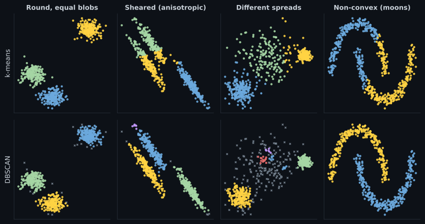
That third column matters. Neither algorithm is universally better; each fails where its assumption is violated. The two later pages in this phase are the detailed versions of these two columns.

In code

import numpy as np
from sklearn.cluster import KMeans
from sklearn.datasets import make_blobs
from sklearn.metrics import (
    calinski_harabasz_score,
    davies_bouldin_score,
    silhouette_score,
)
from sklearn.pipeline import make_pipeline
from sklearn.preprocessing import StandardScaler
 
X, y_true = make_blobs(n_samples=400, centers=4, cluster_std=0.9, random_state=11)
 
# Scaling belongs inside the pipeline, exactly as in supervised work.
model = make_pipeline(StandardScaler(), KMeans(n_clusters=4, n_init=10, random_state=0))
labels = model.fit_predict(X)
 
print("silhouette       ", round(silhouette_score(X, labels), 4))    # 0.7475
print("davies-bouldin   ", round(davies_bouldin_score(X, labels), 4))  # 0.3578, lower is better
print("calinski-harabasz", round(calinski_harabasz_score(X, labels), 1))  # 3241.8

import numpy as np
from sklearn.cluster import KMeans
from sklearn.datasets import make_blobs
from sklearn.metrics import (
    calinski_harabasz_score,
    davies_bouldin_score,
    silhouette_score,
)
from sklearn.pipeline import make_pipeline
from sklearn.preprocessing import StandardScaler
 
X, y_true = make_blobs(n_samples=400, centers=4, cluster_std=0.9, random_state=11)
 
# Scaling belongs inside the pipeline, exactly as in supervised work.
model = make_pipeline(StandardScaler(), KMeans(n_clusters=4, n_init=10, random_state=0))
labels = model.fit_predict(X)
 
print("silhouette       ", round(silhouette_score(X, labels), 4))    # 0.7475
print("davies-bouldin   ", round(davies_bouldin_score(X, labels), 4))  # 0.3578, lower is better
print("calinski-harabasz", round(calinski_harabasz_score(X, labels), 1))  # 3241.8

Note fit_predictfit_predict. Clustering estimators have no yy argument, so fit(X)fit(X) then .labels_.labels_, or fit_predict(X)fit_predict(X) in one step. Only some of them — k-means and Gaussian mixtures — can also predictpredict on unseen rows; DBSCAN and agglomerative clustering cannot, because their labels are defined relative to the training set.

import numpy as np
from sklearn.cluster import KMeans
from sklearn.metrics import adjusted_rand_score
from sklearn.preprocessing import StandardScaler
 
rng = np.random.default_rng(0)
age = np.concatenate([rng.normal(28, 4, 90), rng.normal(52, 4, 90)])
income = np.concatenate([rng.normal(60_000, 12_000, 90), rng.normal(64_000, 12_000, 90)])
X = np.column_stack([age, income])
truth = np.concatenate([np.zeros(90), np.ones(90)])
 
raw = KMeans(n_clusters=2, n_init=10, random_state=0).fit_predict(X)
scaled = KMeans(n_clusters=2, n_init=10, random_state=0).fit_predict(
    StandardScaler().fit_transform(X)
)
 
print("column stds:", X.std(axis=0).round(1))   # [   12.3 12697.7]
print("ARI raw   ", round(adjusted_rand_score(truth, raw), 4))      # 0.0348
print("ARI scaled", round(adjusted_rand_score(truth, scaled), 4))   # 0.8914

import numpy as np
from sklearn.cluster import KMeans
from sklearn.metrics import adjusted_rand_score
from sklearn.preprocessing import StandardScaler
 
rng = np.random.default_rng(0)
age = np.concatenate([rng.normal(28, 4, 90), rng.normal(52, 4, 90)])
income = np.concatenate([rng.normal(60_000, 12_000, 90), rng.normal(64_000, 12_000, 90)])
X = np.column_stack([age, income])
truth = np.concatenate([np.zeros(90), np.ones(90)])
 
raw = KMeans(n_clusters=2, n_init=10, random_state=0).fit_predict(X)
scaled = KMeans(n_clusters=2, n_init=10, random_state=0).fit_predict(
    StandardScaler().fit_transform(X)
)
 
print("column stds:", X.std(axis=0).round(1))   # [   12.3 12697.7]
print("ARI raw   ", round(adjusted_rand_score(truth, raw), 4))      # 0.0348
print("ARI scaled", round(adjusted_rand_score(truth, scaled), 4))   # 0.8914

When you do have labels

Sometimes you have ground truth — you are evaluating a clustering method on a benchmark, or you withheld a label column deliberately. Then use an external score, one that is invariant to how the clusters are numbered.

The adjusted Rand index counts pairs of points that the two labellings agree about (both put them together, or both put them apart), then corrects for the agreement expected by chance:

It is 1.0 for a perfect match, about 0.0 for random labelling, and can go slightly negative. Every comparison in this phase that has a ground truth is reported as an ARI.

Normalised mutual information measures how much knowing one labelling tells you about the other, normalised to $[0, 1]$. It is more forgiving than ARI when one labelling splits a true cluster into several pieces.

Clustering as a feature

A cluster assignment is a categorical feature, and one-hot encoding it can help a supervised model enormously. If you have a regionregion column with 800 distinct values, clustering the region-level statistics into 12 groups gives a supervised model something it can actually learn from.

The same leakage rule as everywhere else applies: the clusterer must be fitted inside the cross-validation fold, on training rows only. KMeansKMeans is a transformer as well as an estimator — its transformtransform returns the distance from each row to each centroid, which is often more useful than the hard label.

from sklearn.cluster import KMeans
from sklearn.linear_model import LogisticRegression
from sklearn.model_selection import cross_val_score
from sklearn.pipeline import make_pipeline
from sklearn.preprocessing import StandardScaler
 
# X and y here are your own supervised dataset.
# KMeans.transform gives k distance columns, which then feed the classifier.
pipe = make_pipeline(
    StandardScaler(),
    KMeans(n_clusters=12, n_init=10, random_state=0),  # acts as a transformer here
    LogisticRegression(max_iter=2000),
)
# cross_val_score refits the KMeans on each training fold — no leakage.
scores = cross_val_score(pipe, X, y, cv=5)

from sklearn.cluster import KMeans
from sklearn.linear_model import LogisticRegression
from sklearn.model_selection import cross_val_score
from sklearn.pipeline import make_pipeline
from sklearn.preprocessing import StandardScaler
 
# X and y here are your own supervised dataset.
# KMeans.transform gives k distance columns, which then feed the classifier.
pipe = make_pipeline(
    StandardScaler(),
    KMeans(n_clusters=12, n_init=10, random_state=0),  # acts as a transformer here
    LogisticRegression(max_iter=2000),
)
# cross_val_score refits the KMeans on each training fold — no leakage.
scores = cross_val_score(pipe, X, y, cv=5)

Pitfalls

Clustering unscaled features. Measured above: ARI 0.035 versus 0.891 on the same data. This is the single most common clustering mistake and it is silent — you get plausible-looking clusters that encode nothing but your unit choices.

Treating the silhouette as truth. It rewards round, equally sized, well-separated clusters. A correct DBSCAN clustering of two moons scores badly on it. Use it to compare similar runs, never to declare one geometry better than another.

Reading meaning into cluster numbers. Cluster 0 in one run is cluster 2 in the next; the labelling is arbitrary and changes with random_staterandom_state. Never join on the raw integer, never write if label == 0if label == 0 in production code. Map clusters to named segments explicitly after inspecting them.

Forgetting that k-means always returns k clusters. Hand it uniform noise and ask for three groups and it will give you three groups, with a silhouette of 0.378 — respectable-looking. Nothing in the algorithm tells you the structure was not there.

Clustering with a distance metric that ignores your categorical columns. One-hot encoding puts every category exactly $\sqrt{2}$ apart in Euclidean space, which is rarely what you mean. Consider Gower distance, or cluster the numeric block and treat the categories separately.

Fitting the scaler on all the data before splitting off a validation set. Clustering feels exploratory so this feels harmless, but the moment the cluster label becomes a feature for a supervised model, it is leakage like any other.

Compare

🧪 Try It Yourself

Exercise 1 – Three metrics on one pair

Exercise 2 – Scaling flips the answer

Exercise 3 – Silhouette by hand, then by sklearn

Exercise 4 – The three internal scores disagree

Exercise 5 – A good clustering that scores badly

Recap

• Clustering has no answer key, so the distance metric is not a detail — it is the definition of the problem.
• Euclidean, Manhattan and cosine gave 5.00, 7.00 and 0.0061 for the same pair of points.
• Scale first. ARI went from 0.035 to 0.891 on identical data with one StandardScalerStandardScaler.
• The silhouette of a point is $(b - a)/\max(a, b)$; negative means misassigned.
• Davies-Bouldin is the one score where lower is better.
• All three internal scores reward round blobs. A perfect DBSCAN clustering of two moons scores 0.329 against k-means’ wrong-but-round 0.479.
• k-means will always return exactly $k$ clusters, including on pure noise.

Exercise 6 – Cluster data that has no clusters

Next

K-Means Clustering Algorithm — Lloyd’s algorithm iteration by iteration, why it always converges but not always well, and the three geometries where it fails outright.