Text Classification with TF-IDF

What you’ll learn

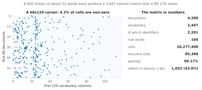
• how a bag of words turns 6,000 short tickets into a 2,447 × 4,200 matrix that is 99.17% zeros
• what idf actually computes, and why the loudest weights go to the least useful tokens
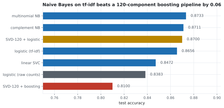
• why sparse linear models win on text: 0.8733 for Naive Bayes against 0.8100 for boosting on 120 SVD components
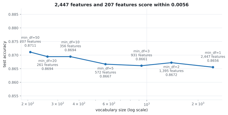
• that min_df=50 deletes 92% of the vocabulary and improves accuracy to 0.8711
• how a template artefact becomes a 5.46 coefficient, and costs 15 accuracy points when the template changes
• when character n-grams beat word n-grams: 0.8611 against 0.8289 on typo’d text

The corpus

Real support tickets cannot be published, so this page uses a synthetic corpus generated from a known process: 6,000 tickets, three queues, about 22 words each. Filler words, a handful of topical words, and a long tail of case identifiers.

the_corpus.py

TOPICS = {
    "billing":   "invoice charged refund payment card ... late lost error".split(),
    "shipping":  "parcel delivery courier tracking ... late lost refund".split(),
    "technical": "login password reset error crash ... charge missing".split(),
}

Three properties are deliberate, and each one shows up in a measurement later:

• The topic vocabularies overlap. refund belongs to billing and shipping; error to billing and technical; late and lost to billing and shipping. This is the irreducible part.
• 6% of the labels are wrong — tickets filed in the wrong queue, as happens.
• 22% of the tokens are case identifiers drawn from a Zipf distribution over 4,000 possible values, which is what makes the matrix wide.

One caveat to state up front: the generator shuffles the words in each document, so word order carries no information by construction. That makes this corpus a clean test of bag-of-words methods and a useless test of anything that depends on sequence — a limitation the n-gram section returns to.

The matrix

figure 6,000 tickets of about 22 words produce a matrix that is 99.17% zeros matplotlib

A document of 22 words can touch at most 22 of 2,447 columns, so the density is bounded by 0.9% before you even look at the data. This is why text features are stored sparse, why linear models are the default, and why 43% of the vocabulary — the tokens that appear in exactly one document — cannot possibly generalise.

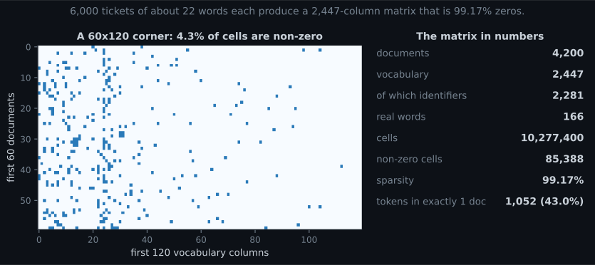
Quantity	Value
training documents	4,200
vocabulary	2,447
of which case identifiers	2,281
actual words	166
non-zero cells	85,388 of 10,277,400
sparsity	99.17%
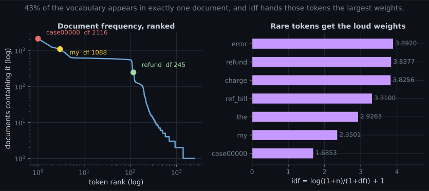
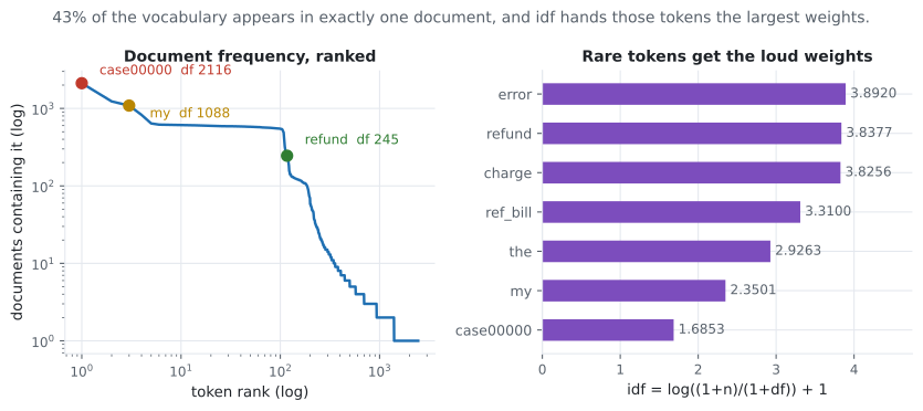
tokens appearing in exactly one document	1,052 (43.0%)

What idf does

Term frequency alone gives every word its raw count. Inverse document frequency down-weights words that appear everywhere. scikit-learn’s smoothed version is

$$\mathrm{idf}(t) = \log\!\frac{1 + n}{1 + \mathrm{df}(t)} + 1, \qquad \mathrm{tfidf}(t, d) = \mathrm{tf}(t, d) \cdot \mathrm{idf}(t)$$

after which each row is L2-normalised, so document length stops mattering.

figure 43% of the vocabulary appears in exactly one document, and idf hands those tokens the largest weights matplotlib

Document frequency follows a power law, so idf spans a narrow range for the common half of the vocabulary and then rises steeply. Note what tops the idf ranking here: not the informative words but whichever ones happen to be rarest. idf is a heuristic about redundancy, not a measure of relevance.

Token	Document frequency	idf
case00000	2,116	1.6853
my	1,088	2.3501
the	611	2.9263
ref_bill	416	3.3100
charge	248	3.8256
refund	245	3.8377
error	232	3.8920

Two things are worth noticing.

The most frequent token is an identifier. case00000 is the head of the Zipf distribution over case numbers and appears in half the documents, so idf treats it as a stopword — correctly, by accident.

idf does not know what matters. error gets the highest weight of the seven above, and it is one of the overlapping words that cannot separate billing from technical. idf measures how unusual a token is, not how diagnostic. Supervised weighting is what the classifier’s coefficients do.

See it move

The idf formula is four operations, and the intuition arrives faster by moving it than by reading it. Toggle which of the eight documents contain the word.

sketch What idf does to a word p5.js Pause Restart

Eight documents; clicking toggles whether each contains the word. The document frequency, the smoothed idf and the resulting tf-idf weight for a document containing the word twice all update from the formula.

Two boundary cases are worth clicking to: a word in all eight documents has idf exactly 1.0000, so tf-idf reduces to term frequency; a word in none of them has no column at all, which is what happens to every token that appears for the first time in production.

Models

figure Naive Bayes on tf-idf beats a 120-component boosting pipeline by 0.06 matplotlib

Every sparse linear method lands between 0.847 and 0.873. Reducing to 120 dense components and applying gradient boosting loses 0.06 — a large amount for this task — because the signal is spread thinly across many weakly informative columns, which is the situation trees handle worst and additive linear models handle best.

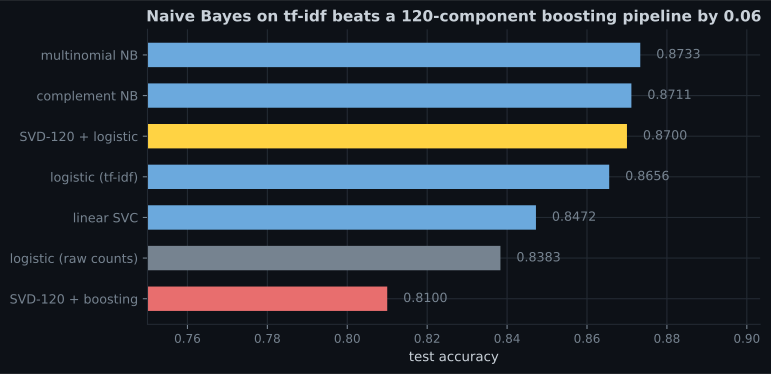
Model	Test accuracy
multinomial Naive Bayes	0.8733
complement Naive Bayes	0.8711
SVD-120 + logistic	0.8700
logistic on tf-idf	0.8656
linear SVC	0.8472
logistic on raw counts	0.8383
SVD-120 + gradient boosting	0.8100

Four things this ordering tells you:

tf-idf is worth 0.0273 over raw counts for the same classifier — a real but modest gain, entirely from down-weighting the identifier tokens that dominate the counts.

Naive Bayes is not a toy. Its independence assumption is false, and it still wins here, in milliseconds, with no hyperparameters. On short documents with sparse features it is the correct baseline and frequently the answer.

Trees are the wrong shape for text. Each split tests one token; discriminating three classes on 1.98 topical words per document needs many weak pieces of evidence added together, which is what a linear model does by construction and what a tree does only with enormous depth.

Dimensionality reduction did not help. SVD-120 + logistic (0.8700) is statistically level with sparse logistic (0.8656) while discarding 2,327 columns and adding a fitted transform to maintain. Reach for it when you need dense vectors for something else, not for accuracy.

The confusion matrix shows where the remaining 13% goes:

true ↓ / predicted →	billing	shipping	technical
billing	523	48	40
shipping	36	520	42
technical	32	44	515

The errors are almost perfectly symmetric — 48 and 36 between billing and shipping, 40 and 32 between billing and technical. Symmetric confusion is the signature of genuinely ambiguous documents (a refund for a damaged parcel belongs to both queues) rather than a model that has learned one class badly.

Most of the vocabulary is dead weight

figure 2,447 features and 207 features score within 0.0056 matplotlib

Raising min_df from 1 to 50 deletes 92% of the columns and the accuracy goes up by 0.0055. Everything discarded was a case identifier appearing in a handful of documents — pure memorisation capacity, no signal. The pruned model is also 12 times smaller and correspondingly faster.

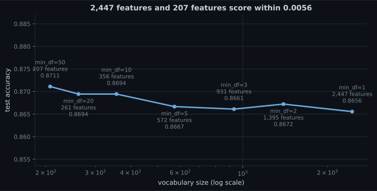
min_df	Vocabulary	Test accuracy
1	2,447	0.8656
2	1,395	0.8672
5	572	0.8667
10	356	0.8694
50	207	0.8711

min_df is the cheapest regularisation available on text, and it is a statement about generalisation rather than about memory: a token that appears in three training documents cannot support a reliable coefficient, and keeping it invites the model to memorise those three.

The companion knob is max_df, which drops tokens appearing in too many documents. On this corpus it does little, because idf already handles them — but on corpora with boilerplate (legal disclaimers, email footers) max_df=0.5 removes a lot of noise in one line.

Two failures that clean cross-validation cannot show you

figure Two failure modes that no cross-validation on clean, same-template data can show you matplotlib

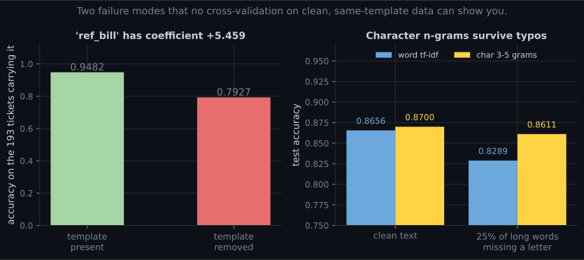
Left: ref_bill is a template artefact carried by 30% of billing tickets. It earns the largest coefficient in the model, +5.459 against +3.173 for the best real word, and when a new ticket system stops emitting it, accuracy on exactly those tickets falls from 0.9482 to 0.7927. Right: deleting one letter from a quarter of the long words costs word-level tf-idf 0.0367 and character n-grams only 0.0089.

The template artefact

30% of billing tickets carry the token ref_bill — a reference-number prefix from the ticketing template, with no meaning whatsoever. The model finds it immediately:

Class	Largest coefficients
billing	ref_bill +5.459, charged +3.173, discount +3.117
shipping	tracking +3.520, address +3.412, warehouse +3.412
technical	bug +3.215, install +3.179, app +3.179

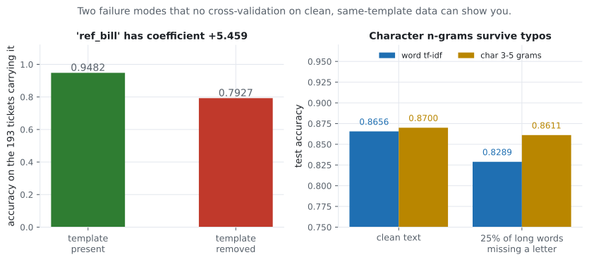
ref_bill outweighs the best genuine billing word by 1.7×, and on the 193 test tickets that carry it the model is right 94.82% of the time against 85.56% elsewhere. Everything looks excellent.

Now migrate the ticketing system so the prefix disappears, and score the same model on the same tickets with that one token removed: 0.7927. A 15.6-point drop, concentrated entirely in the segment that used to be the model’s best.

This is not leakage in the train/test sense — the token is genuinely present at prediction time, and every split reproduces it. It is a dependency on an artefact, and the only defence is reading the coefficients and asking whether each top token is something a human would use to make the same decision. Which is exactly the audit from Phase 09.

Typos, and character n-grams

Word-level features are exact-match: delivery and delivry are unrelated columns. Delete one letter from 25% of the words longer than four characters — a mild simulation of real user text — and word tf-idf falls from 0.8656 to 0.8289. Character n-grams, which see deliv in both spellings, fall only from 0.8700 to 0.8611.

char_ngrams.py

TfidfVectorizer(analyzer="char_wb", ngram_range=(3, 5), min_df=2)
# 7,637 features on this corpus; robust to typos, agglutination and casing

The cost is a wider matrix (7,637 features against 2,447) and features nobody can read. The usual production answer is a FeatureUnion of both: word n-grams for interpretability, character n-grams for robustness.

On n-grams

Features	Vocabulary	Accuracy
unigrams (min_df=2)	1,395	0.8672
unigrams + bigrams	17,634	0.8667
unigrams + bigrams + trigrams	18,543	0.8683

Bigrams add 16,239 columns and 0.0000 of accuracy here — and that result is a property of this corpus, not of text in general. The generator shuffles words, so there are no phrases to find. On real text, bigrams typically buy one to three points on sentiment (“not good”) and almost nothing on topic classification. The lesson is procedural: measure the gain on your corpus before paying for a tenfold wider matrix.

The pipeline

diagram Diagram mermaid

  flowchart TD
  A["Raw documents"] --> B["TfidfVectorizer
lowercase, min_df=2..10"]
  B --> C["Linear model or
Naive Bayes"]
  C --> D{"Beats the majority
class by enough?"}
  D -->|"no"| E["Look at the confusion matrix.
Symmetric = ambiguous labels.
Asymmetric = a broken class."]
  D -->|"yes"| F["Read the top coefficients
per class"]
  F --> G{"Would a human use
these tokens?"}
  G -->|"no — templates,
ids, footers"| H["Remove them and re-measure.
That number is the real one."]
  G -->|"yes"| I["Check robustness:
typos, new vocabulary,
a different template"]
  I --> J["Ship the sparse pipeline.
Pickle the vectorizer WITH
the model."]

The last box is the most common production bug on this page’s subject: a TfidfVectorizer is a fitted object holding the vocabulary and the idf vector. Save the whole Pipeline, never the classifier alone — the same failure, with the same silence, as dropping a scaler.

Pitfalls

Pitfall	Why it bites	What to do
fit_transform on the whole corpus before splitting	The idf vector and vocabulary see the test set	fit on train only, inside a Pipeline
Saving the classifier without the vectorizer	Word IDs mean nothing without the fitted vocabulary	Pickle the whole pipeline
min_df=1 by default	43% of columns appear in one document	min_df=2 minimum; sweep it, 50 was best here
Trusting top coefficients as meaning	ref_bill scored +5.459 and means nothing	Audit them against domain expectation
Adding bigrams reflexively	16,239 extra columns for 0.0000 here	Measure on your corpus first
Exact-match features on user-written text	0.8289 against 0.8611 under mild typos	Add character n-grams
Reaching for boosting on sparse text	0.8100 against 0.8733 for Naive Bayes	Linear first, always
Reading accuracy without the confusion matrix	Symmetric and asymmetric errors need different fixes	Print it every time

Recap

• 6,000 tickets, 22 words each, produced a 2,447-column matrix that is 99.17% zeros, with 43.0% of tokens appearing in exactly one document.
• idf is $\log((1+n)/(1+\mathrm{df})) + 1$: case00000 got 1.6853 and error 3.8920 — it measures rarity, not relevance.
• Multinomial Naive Bayes 0.8733, logistic on tf-idf 0.8656, logistic on raw counts 0.8383, SVD-120 + boosting 0.8100.
• min_df=50 cut the vocabulary by 92% and raised accuracy to 0.8711.
• A meaningless template token earned the model’s largest coefficient (+5.459) and cost 15.6 points on the affected tickets when it disappeared.
• Under mild typos, word features lost 0.0367 and character 3–5 grams 0.0089.
• Bigrams added 16,239 columns and nothing — on this corpus, whose words are shuffled by construction.

pch.quizTag pch.quizDefaultTitle

1. Your document-term matrix is 4,200 x 2,447 and 99.17% zeros. What does that imply about model choice?

   A Use a tree ensemble, which handles sparsity well B Prefer sparse linear models or Naive Bayes: the evidence is spread thinly across many weak columns, which linear models add up and trees cannot C Reduce to 50 dimensions first D It implies nothing about model choice
   pch.quizShowAnswer

   B — Prefer sparse linear models or Naive Bayes: the evidence is spread thinly across many weak columns, which linear models add up and trees cannot — Each tree split tests a single token, and with about two topical words per document no single token is decisive. Measured here: Naive Bayes 0.8733, sparse logistic 0.8656, boosting on 120 SVD components 0.8100.

2. The token with the highest idf in your corpus is a case number. What does that tell you?

   A It is your most informative feature B Nothing about usefulness — idf measures rarity, so the rarest tokens get the loudest weights regardless of whether they discriminate anything C The vectorizer is misconfigured D You should lower max_df
   pch.quizShowAnswer

   B — Nothing about usefulness — idf measures rarity, so the rarest tokens get the loudest weights regardless of whether they discriminate anything — idf is an unsupervised heuristic about redundancy. On this corpus 'error' outranked every informative word while being one of the overlapping tokens that cannot separate billing from technical. Supervised weighting is the classifier's job.

3. Raising min_df from 1 to 50 deletes 92% of your vocabulary and accuracy rises from 0.8656 to 0.8711. Why?

   A Random variation B The deleted tokens appeared in a handful of documents each — pure memorisation capacity with no generalisable signal, so removing them acts as regularisation C The model trains faster and therefore converges better D min_df fixes class imbalance
   pch.quizShowAnswer

   B — The deleted tokens appeared in a handful of documents each — pure memorisation capacity with no generalisable signal, so removing them acts as regularisation — 43% of columns appeared in exactly one training document. A coefficient fitted on one occurrence cannot generalise; deleting those columns loses nothing and constrains the model. The pruned pipeline is also twelve times smaller.

4. The largest coefficient in your billing class is a reference-number prefix from the ticket template. Is that a problem?

   A No — it predicts well on every split B Yes — it works only while the template exists; measured here, accuracy on the affected tickets fell from 0.9482 to 0.7927 when the token was removed C Only if it also appears in other classes D No, provided you keep it out of production
   pch.quizShowAnswer

   B — Yes — it works only while the template exists; measured here, accuracy on the affected tickets fell from 0.9482 to 0.7927 when the token was removed — This is not train/test leakage: the token is genuinely present at prediction time. It is a dependency on an artefact, and it fails silently at the next system migration. Reading the top coefficients and asking whether a human would use them is the only defence.

5. Your model scores 0.87 on clean text and 0.83 on real user submissions full of typos. What is the cheapest fix?

   A Collect more training data B Add character n-grams (analyzer='char_wb', ngram_range=(3, 5)) — they share substrings between 'delivery' and 'delivry', and lost only 0.0089 under the same corruption C Spell-check the inputs at prediction time D Switch to a transformer
   pch.quizShowAnswer

   B — Add character n-grams (analyzer='char_wb', ngram_range=(3, 5)) — they share substrings between 'delivery' and 'delivry', and lost only 0.0089 under the same corruption — Word features are exact-match, so a single deleted letter creates an unseen token and destroys the evidence. Character n-grams degrade gracefully. The usual production shape is a FeatureUnion of word and character features.

🧪 Try It Yourself

Exercise 1 – Generate the corpus

pch.exerciseTag pch.exerciseTitle

Exercise 2 – Vectorize, and look at the matrix

pch.exerciseTag pch.exerciseTitle

Exercise 3 – Fit three models and read the confusion matrix

pch.exerciseTag pch.exerciseTitle

Exercise 4 – Delete 92% of the vocabulary

pch.exerciseTag pch.exerciseTitle

Exercise 5 – Break the template

pch.exerciseTag pch.exerciseTitle

Next

Recommender Systems from Scratch — from a sparse document-term matrix to a sparser user-item matrix, where 99.17% zeros would count as dense and the missing entries are the thing you are trying to predict.