Loss Functions: Choosing What to Minimise

The loss is the only thing a network optimises. Everything else — architecture, optimiser, schedule — is machinery for descending it. Which means a loss that does not match what you care about produces a model that is excellent at the wrong thing, and no amount of tuning fixes that.

What you’ll learn

Why the derivative of the loss matters more than the loss, and what MSE, MAE and Huber’s derivatives look like.
Huber implemented from scratch and matched to Keras at 0.00e+00.
The measured cost of MSE on contaminated targets: 0.3116 against 0.2279 MAE on clean data.
Why cross-entropy pairs with sigmoid and softmax — the gradient reduces to $\hat{y} - y$ .
What from_logits=True prevents: a loss reported as 16.118095 instead of 40.0, with a gradient of exactly zero.
Class weights on a 20:1 imbalance: recall 0.5482 → 0.7665.
Label smoothing measured, including the run where smoothing 0.2 was the most accurate as well as the least over-confident.

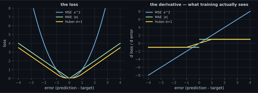
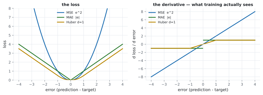
The loss is a choice, the derivative is the consequence

Training never looks at the loss value. It looks at $\partial L / \partial \theta$ , and every property that matters follows from that derivative.

Two panels. Left: MSE as a steep parabola, MAE as a V, and Huber tracking MSE near zero then continuing as straight lines. Right: their derivatives — MSE a straight line growing without bound, MAE a step from minus one to plus one with a gap at zero, Huber a ramp that saturates at plus or minus one. — On the left the three look broadly similar. On the right they are completely different: MSE's derivative grows without limit, so one large error dominates every update. MAE's derivative is a constant ±1 — every error pulls equally hard, and there is no derivative at all at zero. Huber's derivative is MSE's near the origin and MAE's beyond δ, which is exactly the design goal.

\text{MSE} = e^2 \qquad \text{MAE} = \lvert e \rvert \qquad \text{Huber}_\delta = \begin{cases} \tfrac{1}{2} e^2 & \lvert e \rvert \le \delta \\ \delta\left(\lvert e \rvert - \tfrac{1}{2}\delta\right) & \text{otherwise} \end{cases}

Error $e$	MSE	MAE	Huber (δ=1)	$\partial$ MSE	$\partial$ MAE	$\partial$ Huber
0.1	0.0100	0.1000	0.0050	0.20	1.00	0.10
1.0	1.0000	1.0000	0.5000	2.00	1.00	1.00
5.0	25.0000	5.0000	4.5000	10.00	1.00	1.00
20.0	400.0000	20.0000	19.5000	40.00	1.00	1.00

At an error of 20, MSE’s gradient is 40 and Huber’s is 1. That is a factor of 40 difference in how hard a single bad row pulls the weights.

Take five errors, $[0.5, -0.5, 1.0, -1.0, 20.0]$ :

Loss	Mean value	Share contributed by the single 20.0 error
MSE	80.5000	0.9938
MAE	4.6000	0.8696
Huber δ=1	4.1500	0.9398

MSE hands 99.4% of the signal to one row out of five.

Measured: what that costs

600 points on the line $y = 2x + 1$ with mild noise, then 30 of them (5%) contaminated with standard-deviation-25 noise. Fit a single Dense(1) with each loss and check the learned parameters against the truth:

Loss	Learned slope (true 2.0)	Learned bias (true 1.0)	MAE against the clean targets
MSE	2.0881	0.7584	0.3116
MAE	2.0117	0.9754	0.2279
Huber δ=1	1.9922	0.9756	0.2282

MSE’s bias lands 0.24 low because it is still trying to reach the outliers. MAE and Huber are within 0.0003 of each other and both recover the true line. Five percent contamination cost MSE 37% more error than either robust loss.

The catch, and the reason MSE remains the default: MAE’s derivative is discontinuous at zero and constant everywhere else, so it converges more slowly and can oscillate around the minimum with a fixed learning rate. Huber gives you MAE’s robustness with MSE’s smooth behaviour near the optimum — at the cost of one extra hyperparameter, $\delta$ .

diagram Diagram mermaid

  flowchart TD
  A["what kind of target?"] --> B{"continuous number"}
  A --> C{"one of K classes"}
  B --> D{"outliers present?"}
  D -- "no" --> E["mse
smooth, fast, standard"]
  D -- "yes" --> F["huber(delta)
or mae if you want
no extra knob"]
  C --> G{"how many classes?"}
  G -- "2" --> H["binary_crossentropy
sigmoid output, 1 unit"]
  G -- "K > 2, one label" --> I["sparse_categorical_crossentropy
softmax output, K units"]
  G -- "K > 2, many labels" --> J["binary_crossentropy
sigmoid output, K units"]

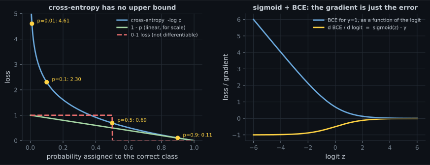
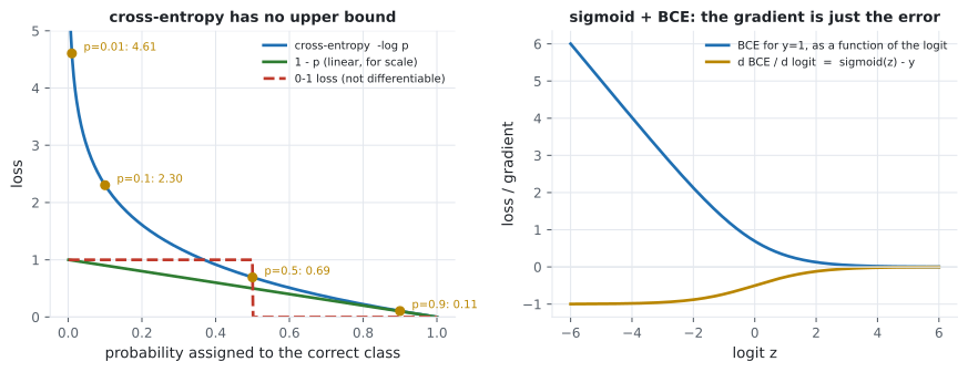
Cross-entropy, and why it pairs with sigmoid and softmax

For classification the loss is the negative log of the probability the model gave the correct answer:

L = -\log \hat{p}_{\text{true class}}

Two panels. Left: negative log p rising steeply toward infinity as p approaches zero, against a linear 1-minus-p line and a step-shaped 0-1 loss. Right: binary cross-entropy as a function of the logit, alongside its derivative, which is a sigmoid curve shifted down by one. — Left: at p=0.9 the loss is 0.11; at p=0.01 it is 4.61. A linear penalty would have moved from 0.1 to 0.99. Right: differentiate binary cross-entropy with respect to the logit and everything cancels — the gradient is sigmoid(z) − y, the plain prediction error. That cancellation is why sigmoid pairs with BCE and softmax pairs with categorical cross-entropy.

$\hat{p}$ assigned to the truth	Loss
0.99	0.010050
0.90	0.105361
0.50	0.693147
0.10	2.302585
0.01	4.605170
0.001	6.907755

Verified against Keras on four rows:

Row	$\hat{p}$ (truth)	$-\log \hat{p}$	Keras
0	0.7000	0.356675	0.356675
1	0.8000	0.223144	0.223144
2	0.4000	0.916291	0.916291
3	0.0200	3.912023	3.912023

Mean 1.352033 both ways, difference 0.00e+00. Row 3 — the confident mistake — contributes 72.3% of the total.

The cancellation

For a sigmoid output $\hat{y} = \sigma(z)$ and binary cross-entropy:

\frac{\partial L}{\partial z} = \frac{\partial}{\partial z}\Big[-y\log\sigma(z) - (1-y)\log(1-\sigma(z))\Big] = \sigma(z) - y

The $\sigma'(z) = \sigma(z)(1-\sigma(z))$ term that would saturate cancels exactly against the $1/\sigma(z)$ from the log. The gradient is the prediction error and nothing else — no saturation, no vanishing, however wrong the model is. Pair sigmoid with MSE instead and that cancellation does not happen; a confidently wrong sigmoid output has a near-zero derivative and learns nothing.

`from_logits=True` is not a style preference

Two mathematically identical routes to the same number:

Output a softmax, then take the log inside the loss.
Output raw logits and let the loss do both at once, using the log-sum-exp trick derived on the Reuters page.

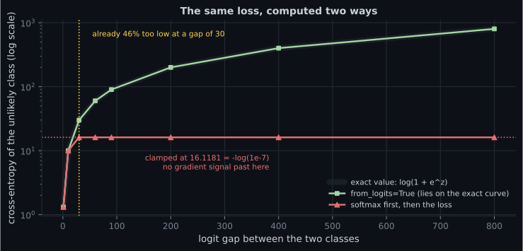
Log-scale plot of cross-entropy against the logit gap between two classes. The exact curve and the from_logits curve lie on top of each other and grow linearly with the gap. The naive softmax-then-loss curve tracks them until a gap of about ten and then flattens permanently at 16.118. — Up to a logit gap of 10 the two agree to six digits. At a gap of 30 the naive path returns 16.118095 instead of 30 — 46% too low. Past that it never moves again, because Keras clips probabilities to 1e-7 and −log(1e-7) = 16.118095. The from_logits path tracks the exact value all the way to a gap of 800.

Logit gap	Exact $\log(1+e^z)$	`from_logits=True`	softmax first	softmax’s $p_0$
1	1.313262	1.313262	1.313262	2.689e−01
10	10.000045	10.000046	10.000046	4.540e−05
30	30.000000	30.000000	16.118095	9.358e−14
90	90.000000	90.000000	16.118095	0.000e+00
800	800.000000	800.000000	16.118095	0.000e+00

At a gap of 90 the softmax probability underflows to exactly zero in float32. The loss then reports a finite 16.118095, so nothing looks broken. The real damage is one level down:

Route	Loss at logits `[0, 40]`, true class 0	$\partial L / \partial z$
`from_logits=True`	40.000000	`[-1.0, 1.0]`
softmax, then the loss	16.118095	`[0.0, 0.0]`

The gradient is exactly zero. The model is maximally wrong about this example and receives no signal at all to fix it — the clipping that kept the loss finite also flattened the function. No error is raised, no nan appears in the logs, and training simply ignores those rows forever.

Two equivalent-looking models; only one is safe

# fine on well-behaved data, silently broken on confident mistakes
model = keras.Sequential([..., keras.layers.Dense(10, activation="softmax")])
model.compile("adam", "sparse_categorical_crossentropy")
 
# preferred: the loss owns the normalisation
model = keras.Sequential([..., keras.layers.Dense(10)])          # no activation
model.compile("adam", keras.losses.SparseCategoricalCrossentropy(
    from_logits=True))

Applying softmax and from_logits=True is the mirror-image bug: the loss then exponentiates already-normalised probabilities. Pick exactly one.

sketch Move the prediction, watch four losses p5.js

Drag the prediction marker. MSE, MAE, Huber and cross-entropy are computed live for a target of 1.0, so you can see which loss reacts to which kind of error.

Weighting the loss when the classes are not balanced

A 20:1 binary problem built from Fashion-MNIST: 747 t-shirts against 37 shirts in training, and a balanced 200/197 test set.

	Accuracy	Recall	Precision	Predicted positive
no weights	0.7733	0.5482	0.9908	109 of 397
`class_weight` balanced	0.8489	0.7665	0.9152	165 of 397

Without weighting the model finds nearly every shirt it predicts (precision 0.9908) but misses 45% of them. Weighting the rare class by $747/37 = 20.2$ raises recall by 0.218 and costs 0.076 of precision.

One argument, applied inside the loss

counts = np.bincount(y_train.astype(int))
weights = {i: len(y_train) / (len(counts) * count)
           for i, count in enumerate(counts)}
model.fit(x_train, y_train, class_weight=weights)

class_weight multiplies each example’s loss term. That is all it does — no resampling, no change to the data. Two consequences worth knowing: gradient magnitudes grow with the weights, so an aggressive weighting can require a lower learning rate; and accuracy stops being comparable across weightings, because you have deliberately told the model that the two error types cost different amounts.

Label smoothing

Instead of asking for probability 1.0 on the true class, ask for $1 - \varepsilon$ and spread $\varepsilon$ across the rest. Measured on Fashion-MNIST, 8,000 rows, 15 epochs, identical seeds:

Smoothing	Test accuracy	Mean confidence	Confidence − accuracy	Confidence when wrong
0.00	0.8445	0.8647	+0.0202	0.6700
0.05	0.8380	0.8048	−0.0332	0.5841
0.10	0.8370	0.7588	−0.0782	0.5496
0.20	0.8550	0.6847	−0.1703	0.4890

The confidence-minus-accuracy gap is a calibration measure: positive means the model is more sure than it deserves to be. Unsmoothed, this model is over-confident by 0.02 and still averages 0.67 confidence on predictions that are wrong. Smoothing fixes that, and by 0.2 it over-corrects into under-confidence by 0.17.

The honest surprise is the accuracy column. Smoothing 0.2 was the most accurate setting in this run, not the least — while 0.05 and 0.10 were both slightly worse than no smoothing at all. The usual framing, “label smoothing trades a little accuracy for better calibration”, does not describe what happened here. On a single 2,000-row test set these differences (0.8370 to 0.8550) are within the range several seeds would produce anyway, which is the real lesson: treat a 0.01-level accuracy difference as unmeasured until you have run it several times.

sketch The measured table, ranked p5.js

Click a column to rank every row by it. The bars are that column's values and the highest and lowest are computed from the numbers, not written in.

Pitfalls

Using softmax with from_logits=False on confident predictions. The loss clamps at 16.118095 and the gradient becomes exactly zero. Prefer raw logits plus from_logits=True.
Applying softmax and from_logits=True. The loss then normalises twice. Exactly one of the two should do it.
Pairing sigmoid with MSE for classification. The saturating derivative no longer cancels, so confidently wrong outputs stop learning.
Reaching for MSE on data with outliers. Five percent contamination cost 37% more error here than Huber.
Reporting MSE as if it were in the target’s units. It is in squared units; take the square root or report MAE.
Comparing accuracy across different class_weight settings. You changed the objective, so the metric is no longer measuring the same thing.
Treating a 0.01 accuracy difference as a result. The label-smoothing table above is a live example of noise looking like signal.
Choosing a loss to match the metric you report. Some metrics (accuracy, F1, AUC) have no useful gradient. Train on a differentiable surrogate, report the metric you care about, and keep the two straight.

Recap

Training sees the derivative, not the loss. MSE’s derivative grows without bound, MAE’s is a constant ±1, Huber’s switches between them at δ.
On 5% contaminated targets, MSE’s clean-data MAE was 0.3116 against 0.2279 for MAE and 0.2282 for Huber.
Cross-entropy is $-\log \hat{p}_{\text{true}}$ , unbounded as the probability approaches zero; one confident error contributed 72.3% of a four-row loss.
Sigmoid + BCE and softmax + cross-entropy exist because the saturating term cancels, leaving a gradient of $\hat{y} - y$ .
from_logits=True is a correctness requirement, not a style choice: the naive path returned 16.118095 instead of 40.0 with a gradient of exactly zero.
class_weight scales each example’s loss term; on a 20:1 imbalance it moved recall from 0.5482 to 0.7665 at a cost of 0.076 precision.
Label smoothing reliably reduced over-confidence; its effect on accuracy here was within noise, and 0.2 happened to score highest.

With the objective settled, the question becomes how to descend it — and the answer is more interesting than “use Adam”: Backpropagation and Optimizers.

pch.quizTag pch.quizDefaultTitle

A model outputs softmax probabilities and the loss is compiled with from_logits=False. On an example where the correct class receives a probability of 4e-18, what happens?

pch.quizShowAnswer

B — The loss is clipped to 16.118095 = -log(1e-7) and the gradient becomes exactly zero, so the model receives no signal from that example and nothing appears wrong in the logs — Silent zero gradients are worse than a crash. Output raw logits and pass from_logits=True.
Why does cross-entropy pair with sigmoid rather than MSE?

pch.quizShowAnswer

B — Differentiating BCE through a sigmoid cancels the saturating sigmoid'(z) term, leaving a gradient of sigmoid(z) - y — the plain error — so confidently wrong predictions still produce a large gradient — With MSE the sigmoid derivative survives, so a confidently wrong output has a near-zero gradient and stops learning.
On 5% contaminated targets, MSE learned a bias of 0.7584 where the truth was 1.0, while Huber learned 0.9756. What causes the difference?

pch.quizShowAnswer

B — MSE's derivative grows linearly with the error, so the 30 contaminated rows contribute gradients tens of times larger than clean rows and pull the fit toward them — At an error of 20 the MSE gradient is 40 and Huber's is 1 — a 40x difference in pull from a single row.
What exactly does class_weight={0: 1.0, 1: 20.2} do?

pch.quizShowAnswer

B — It multiplies each example's loss term by its class's weight — nothing is resampled, and gradient magnitudes grow accordingly — Because gradients grow with the weights, an aggressive weighting can need a lower learning rate; and accuracy is no longer comparable to the unweighted run.
In the measured label-smoothing table, accuracy went 0.8445, 0.8380, 0.8370, 0.8550 for smoothing 0, 0.05, 0.1, 0.2. What is the right conclusion?

pch.quizShowAnswer

B — The calibration effect is large and consistent, but the accuracy differences are small enough on a 2,000-row test set that they should be treated as noise until repeated across seeds — The confidence gap moved monotonically from +0.0202 to -0.1703. Accuracy did not, and single-run differences of 0.01 are not results.

🧪 Try It Yourself

pch.coffeeTagline

pch.coffeeCta

pch.feedbackHeading

pch.feedbackSubheading